IT-9-O-2387 Retrieving nanoscale third-dimension information directly from TEM data using stacked-Bloch-wave simulations and artificial neural network tools
Transmission electron microscope (TEM) specimens are three-dimensional, but TEM images and diffraction patterns are two-dimensional. To retrieve the "third-dimensional" information, we have developed a direct-retrieval algorithm including dynamical diffraction that can use TEM data (such as a single convergent-beam electron diffraction [CBED] pattern) and retrieve variations of a range of nanoscale specimen parameters, including strain, crystal tilt, and chemical composition. The retrieval algorithm itself is detailed elsewhere [1], and uses the stacked-Bloch-wave algorithm [2-3] and artificial neural network optimization tools [4]. In this work, we show the effectiveness of our algorithm and discuss considerations for applying this algorithm to realistic experimental data.
A demonstration of this algorithm’s third-dimension (depth-dependent) retrieval ability is seen in Figures 1 & 2. Figures 1 and 2 show CBED patterns of a 100-nm-thick Si specimen at 80 kV at the [110] zone axis, simulated using the stacked-Bloch-wave [2-3] forward-simulation algorithm and 197 zero-order-Laue-zone reflections. Figure 1 has "asymmetric" diffraction features due to the third-dimension variation of crystal tilt. Figure 2 is a CBED pattern like that in Figure 1 but without third-dimension variation, and fails to reproduce the correct diffraction features. Figures 3 and 4 demonstrate our algorithm’s effective and accurate retrieval of third-dimension variation in crystal tilt (Δα, mean over all layers) from the specimen shown in Figure 1a, and decreasing mismatch between simulated and experimental CBED intensity (given by ΔE, mean over all reciprocal-space points). Figure 4 shows how well the unknown α is determined for a known E mismatch.
This algorithm can retrieve third-dimension material properties from a single CBED pattern; however, other techniques like dark-field image series or large-angle rocking-beam electron diffraction (LARBED) series can also be used. Each technique has its own advantages and challenges, especially for analysis of strain or compositional variations. Large lattice-parameter variations can also require a modification to the algorithm in [1].
In this work, we present practical considerations for using our third-dimension information-retrieval algorithm [1]. We demonstrate its effectiveness, discuss different acquisition techniques and consider how different parameters affect our algorithm.
[1]: R. S. Pennington, W. Van den Broek, C. T. Koch. (submitted)
[2]: R. S. Pennington, F. Wang, C. T. Koch. Ultramicroscopy, 2014. http://dx.doi.org/10.1016/j.ultramic.2014.03.003
[3]: D. J. Eaglesham, C. J. Kiely, D. Cherns, and M. Missous. Phil. Mag. A 60, 161
(1989).
[4]: R. Rojas. Neural Networks: A Systematic Introduction (Springer Verlag, Berlin, 1993).
We acknowledge funding from the Carl Zeiss Foundation and Grant No. KO 2911/7-1 of the German Research Foundation (DFG).
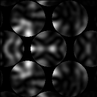
Fig. 1: Simulated zero-loss-filtered convergent-beam electron diffraction (CBED) pattern, generated from a specimen with third-dimension crystal tilt variation. The specimen has ten 10 nm layers, tilted along the [001] direction {0.00, -0.04, -0.10, -0.20, -0.30, -0.30, -0.20, -0.14, -0.06, 0.00} degrees, respectively. |

Fig. 2: A CBED pattern like Figure 1, but generated from a specimen with no layer-by-layer crystal tilt variation but with the same mean crystal tilt, which fails to reproduce the "asymmetric" diffraction features seen. |
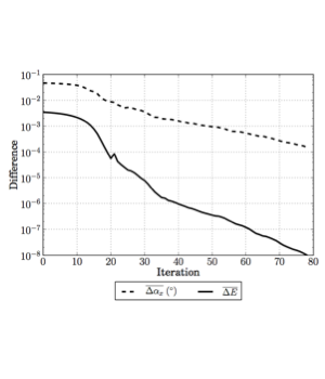
Fig. 3: Our algorithm [1] retrieves third-dimensional variation in crystal tilt (see text) using a (13x13) point reciprocal-space grid, each point 0.05 degrees apart, starting at the 000 point and moving in the [001] and [-110] directions. (This area does not correspond to the discs in Figure 1, but is from the same specimen.) |
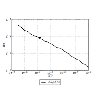
Fig. 4: The unknown third-dimension parameter mismatch (Δα, mean over all layers), plotted as a function of the known intensity mismatch (ΔE, mean over all points). |