IT-11-P-2006 Solving the transport of intensity equation using flux-preserving boundary conditions
The Transport of Intensity Equation (TIE) is a non-interferometric phase reconstruction method which overcomes disadvantages of interferometric methods such as coherent illumination and interferometer stability [1]. The TIE is a Poisson type equation which relates a modified Laplacian of the phase of the wave to the intensity variation along the optical axis (see eqn.(a.1) in Fig 1). In the absence of singularities in the principle (central) plane of focus, many approaches of solving the TIE exist. The problem common to all these approaches is that the necessary boundary conditions are not known. The most popular approach is based on the Fast Fourier Transform (FFT) and solves the TIE non-iteratively in the frequency domain. The implicitly assumed periodic boundary conditions are the main drawback of this method [1]. Another method is based on the multigrid approach for solving partial differential equations, yielding an exact solution of the TIE in the spatial domain. This approach allows us to define zero-flux boundary conditions (Fig1,eq. (a.2), where n ⃑ is the normal to the boundary) and the a vanishing phase shift within regions of vacuum. Since the phase in vacuum is constant, a circle (the number or the shape is arbitrary) with Dirichlet boundary condition can be placed in an area containing vacuum. Figure 1b shows the graphical representation of above-mentioned boundary conditions. Fig.2a and b show under and over focused images which are used to compute the intensity variation along the optical axis (Fig.2c).
Fig. 3 compares phase maps reconstructed from the simulated data by different methods. Fig. 3c shows the phase recovered by the Fourier method and our finite element multigrid solution obtained by using the software package COMSOL is shown in Fig. 3b. This figure shows clearly that especially the low frequency details of the phase reconstructed by the flux-preserving approach agree better with the phase used for simulating the images, than the reconstruction obtained by the Fourier transform method. In our presentation we will show applications of this method to experimental data acquired in the TEM and also the optical microscope.
[1] D. Paganin and K.A. Nugent, Non-interferometric phase imaging with partially-coherent light Phys. Rev. Lett., 80, 2586-2589 (1998)
This work was supported financially by the Carl Zeiss Foundation as well as the German Research Foundation (DFG, Grant No. KO 2911/7-1).
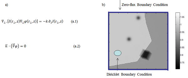
Fig. 1: a) (a.1)TIE equation and (a.2) Equation defining the zero-flux boundary condition b) Graphical representation of the combination of boundary conditions used for the reconstruction scheme presented here. |
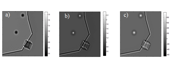
Fig. 2: Under-focused image b) Over-focused image c) dI/dz approximated by the difference of the images shown in a and b. |
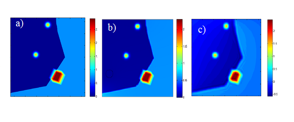
Fig. 3: a) Original phase, b) Phase reconstructed by the method presented here c) Phase reconstructed by the FFT method for solving the TIE. |
|