IT-11-P-1727 Observation of Magnetic Field by Combination of Electron Tomography and Holography
Electron tomography has developed in the last decade with the progress of electron microscopy and the development of algorithms for the Radon transformation and image processing with interpolation [1]. On the other hand, electron holography is one of the standard techniques for observing phase maps of electron waves. The combination of tomography and holography has also led to elucidation of the distributions of the mean inner potential of materials [2]. In the case of the magnetic field, the component By parallel to the rotation axis (see Fig. 1(a)) can be calculated from the phase shift Δφy by using the conventional tomography algorithm [3], but the other two components (Bx, Bz) perpendicular to the rotation axis cannot be calculated, because they are mixed together with a rotation angle θ. In the case of a magnetic field in free space, however, the phase shift Δφθ projected to the optical axis can be described simply [4], for which Bx and Bz can be separated.
Figure 1(a) is a schematic diagram of the tomography/holography experiment. A thin magnetic pillar made of C/CoFeB/SiO2 was prepared with a focused ion beam machine (see Fig. 1(b)) and mounted on the 360° rotation axis of the specimen holder. Two holograms projected from the front surface and back surface of the material were processed in order to divide the magnetic and electric fields around the specimen. Figures 1(c) and (d) are examples of reconstructed interferograms of the magnetic and electric fields. Holograms made with a double-biprism interferometer [5] for tomography were recorded every 10°. Eighteen phase maps corresponding to the projected magnetic field were reconstructed from thirty-six holograms. The phase maps were processed into a three-dimensional (3-D) magnetic field distribution in free space by using a modified tomography algorithm.
Figure 2 shows the reconstructed 3-D magnetic field distribution on the plane perpendicular to the pillar-shaped magnet. Figure 3 shows the reconstructed magnetic field in three planes parallel to the pillar.
To improve the precision and resolution of 3-D reconstructions of the magnetic field, especially inside the material, the two components of the magnetic field should be measured independently. A dual-axis 360° rotation specimen holder has already been developed for this purpose [6]. The results of an experiment using this dual-axis holder will be reported soon.
References:
[1] S. Ono et al., Appl. Phys. Express, 4, (2011) 066601.
[2] G. Lai et al., Appl. Opt., 33, (1994) 829.
[3] G. Lai et al., J. Appl. Phys., 75, (1994) 4593.
[4] H. Shinada et al., IEEE Transaction on Magnetics, 28, (1992) 1017.
[5] K. Harada et al., Appl. Phys. Lett., 84, (2004) 3229.
[6] R. Tsuneta et al., Kenbikyou, 48, (2013) 205 (in Japanese).
The authors would like to thank Mr. H. Hasegawa of the Central Research Lab., Hitachi Ltd. for supplying the C/CoFeB/SiO2 specimens and valuable discussion.
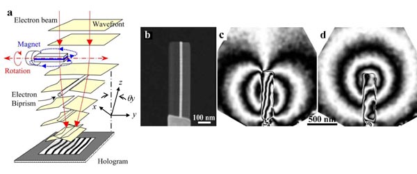
Fig. 1: (a) Experimental setup for tomography/holography, (b) scanning ion micrograph of C/CoFeB/SiO2 pillar, (c) reconstructed interferogram of magnetic field, (d) interferogram of electric field. |
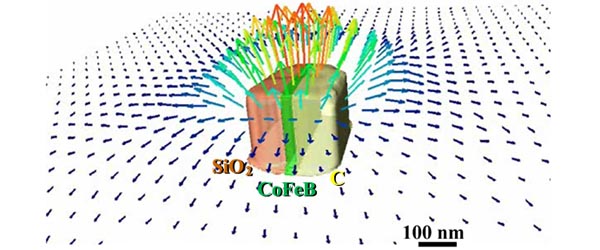
Fig. 2: Reconstructed 3-D magnetic field distribution in one horizontal plane. |
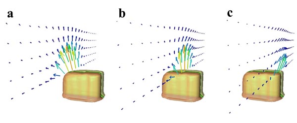
Fig. 3: Reconstructed 3-D magnetic field distributions in three vertical planes (a, b and c). |
|